Creating, reading, and writing reference
This is the reference component to the "Creating, reading, and writing" section of the tutorial. For the workbook section, click here.
The very first step in any data analytics project will probably reading the data out of a file somewhere, so it makes sense that that's the first thing we'd need to cover. In this section, we'll look at exercises on creating pandas Series and DataFrame objects, both by hand and by reading data from disc.
The IO Tools section of the official pandas docs provides a comprehensive overview on this subject.
import pandas as pd
Creating data
There are two core objects in pandas: the DataFrame and the Series.
A DataFrame is a table. It contains an array of individual entries, each of which has a certain value. Each entry corresponds with a row (or record) and a column.
For example, consider the following simple DataFrame:
pd.DataFrame({'Yes': [50, 21], 'No': [131, 2]})
In this example, the "0, No" entry has the value of 131. The "0, Yes" entry has a value of 50, and so on.
DataFrame entries are not limited to integers. For instance, here's a DataFrame whose values are str strings:
pd.DataFrame({'Bob': ['I liked it.', 'It was awful.'], 'Sue': ['Pretty good.', 'Bland.']})
We are using the pd.DataFrame constructor to generate these DataFrame objects. The syntax for declaring a new one is a dictionary whose keys are the column names (Bob and Sue in this example), and whose values are a list of entries. This is the standard way of constructing a new DataFrame, and the one you are likliest to encounter.
The dictionary-list constructor assigns values to the column labels, but just uses an ascending count from 0 (0, 1, 2, 3, ...) for the row labels. Sometimes this is OK, but oftentimes we will want to assign these labels ourselves.
The list of row labels used in a DataFrame is known as an Index. We can assign values to it by using an index parameter in our constructor:
pd.DataFrame({'Bob': ['I liked it.', 'It was awful.'],
              'Sue': ['Pretty good.', 'Bland.']},
             index=['Product A', 'Product B'])
A Series, by contrast, is a sequence of data values. If a DataFrame is a table, a Series is a list. And in fact you can create one with nothing more than a list:
pd.Series([1, 2, 3, 4, 5])
A Series is, in essence, a single column of a DataFrame. So you can assign column values to the Series the same way as before, using an index parameter. However, a Series do not have a column name, it only has one overall name:
pd.Series([30, 35, 40], index=['2015 Sales', '2016 Sales', '2017 Sales'], name='Product A')
Series and the DataFrame are intimately related. It's helpful to think of a DataFrame as actually being just a bunch of Series "glue together". We'll see more of this in the next section of this tutorial.
Reading common file formats
Being able to create a DataFrame and Series by hand is handy. But, most of the time, we won't actually be creating our own data by hand, we'll be working with data that already exists.
Data can be stored in any of a number of different forms and formats. By far the most basic of these is the humble CSV file. When you open a CSV file you get something that looks like this:
csv
Product A,Product B,Product C,
30,21,9,
35,34,1,
41,11,11
So a CSV file is a table of values separated by commas. Hence the name: "comma-seperated values", or CSV.
Let's now set aside our toy datasets and see what a real dataset looks like when we read it into a DataFrame. We'll use the read_csv function to read the data into a DataFrame. This goes thusly:
wine_reviews = pd.read_csv("../input/wine-reviews/winemag-data-130k-v2.csv")
We can use the shape attribute to check how large the resulting DataFrame is:
wine_reviews.shape
So our new DataFrame has 130,000 records split across 14 different columns. That's almost 2 million entries!
We can examine the contents of the resultant DataFrame using the head command, which grabs the first five rows:
wine_reviews.head()
The pandas read_csv function is well-endowed, with over 30 optional parameters you can specify. For example, you can see in this dataset that the csv file has an in-built index, which pandas did not pick up on automatically. To make pandas use that column for the index (instead of creating a new one from scratch), we may specify and use an index_col.
wine_reviews = pd.read_csv("../input/wine-reviews/winemag-data-130k-v2.csv", index_col=0)
wine_reviews.head()
Let's look at a few more datatypes you're likely to encounter.
First up, the venerable Excel spreadsheet. An Excel file (XLS or XLST) organizes itself as a sequence of named sheets. Each sheet is basically a table. So to load the data into pandas we need one additional parameter: the name of the sheet of interest.
So this:
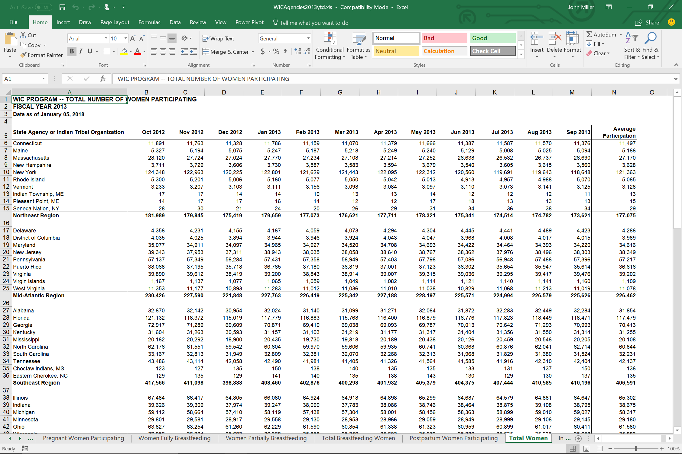
Becomes this:
wic = pd.read_excel("../input/xls-files-all/WICAgencies2013ytd.xls",
                    sheet_name='Total Women')
wic.head()
As you can see in this example, Excel files are often not formatted as well as CSV files are. Spreadsheets allow (and encourage) creating notes and fields which are human-readable, but not machine-readable.
So before we can use this particular dataset, we will need to clean it up a bit. We will see how to do so in the next section.
For now, let's move on to another common data format: SQL files.
SQL databases are where most of the data on the web ultimately gets stored. They can be used to store data on things as simple as recipes to things as complicated as "almost everything on the Kaggle website".
Connecting to a SQL database requires a lot more thought than reading from an Excel file. For one, you need to create a connector, something that will handle siphoning data from the database.
pandas won't do this for you automatically because there are many, many different types of SQL databases out there, each with its own connector. So for a SQLite database (the only kind supported on Kaggle), you would need to first do the following (using the sqlite3 library that comes with Python):
import sqlite3
conn = sqlite3.connect("../input/188-million-us-wildfires/FPA_FOD_20170508.sqlite")
The other thing you need to do is write a SQL statement. Internally, SQL databases all operate very differently. Externally, however, they all provide the same API, the "Structured Query Language" (or...SQL...for short).
We (very briefly) need to use SQL to load data into
For the purposes of analysis however we can usually just think of a SQL database as a set of tables with names, and SQL as a minor inconvenience in getting that data out of said tables.
So, without further ado, here is all the SQL you have to know to get the data out of SQLite and into pandas:
fires = pd.read_sql_query("SELECT * FROM fires", conn)
Every SQL statement beings with SELECT. The asterisk (*) is a wildcard character, meaning "everything", and FROM fires tells the database we want only the data from the fires table specifically.
And, out the other end, data:
fires.head()
Writing common file formats
Writing data to a file is usually easier than reading it out of one, because pandas handles the nuisance of conversions for you.
We'll start with CSV files again. The opposite of read_csv, which reads our data, is to_csv, which writes it. With CSV files it's dead simple:
wine_reviews.head().to_csv("wine_reviews.csv")
To write an Excel file back you need to_excel and the sheet_name again:
wic.to_excel('wic.xlsx', sheet_name='Total Women')
And finally, to output to a SQL database, supply the name of the table in the database we want to throw the data into, and a connector:
conn = sqlite3.connect("fires.sqlite")
fires.head(10).to_sql("fires", conn)
Painless!